Deep Learning :

To understand “Deep Learning” first let us try to understand how it is related to AI and Machine Learning. Look at the given figure :

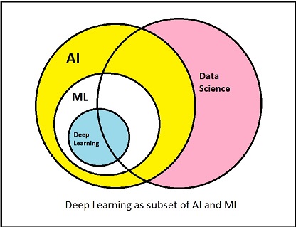
From this figure we can clearly understand the importance of deep learning as a subset of AI.

Deep Learning is learning the deep, in-depth patterns and important features of a dataset. Dataset here means the collection of different kinds of data that we want to study and, predict a result from. The history of Deep Learning can be traced back to 1943 when Walter Pitts and Warren McCulloch created a computer model based on the neural networks of the human brain.

This blog deals with the basic understanding of how a Neural network works.

So now, we have a rough idea about what deep learning is and from it, we can surely understand why it is important. Now let's move forward to understanding Neural Networks.

Neural Networks :

Deep Learning is a very important idea, and to make this idea go on track, we have to use Neural Networks. Neural Networks, in this case, the Artificial Neural Networks (ANNs) more precisely, are similar to biological neurons in our human body. Neurons as in a human body are responsible for transmitting the information of stimulus like touch, similarly, the artificial neuron (Every single unit in a neural network is called a neuron) transmits information learned by every neuron to the next neuron in another layer or different similar neurons.

This is the easiest way to understand what a set of neurons does. Let’s dive deeper and understand how these neural networks are made and how they get their job done. Neurons in artificial neural networks (ANNs) are sometimes even referred to as “nodes”.

The first artificial neural network was invented in 1958 by psychologist Frank Rosenblatt, called Perceptron. It was intended to model how the human brain processed visual data and learned to recognize objects. This model was made with interconnected wires to transfer information between them, but today's neural networks don’t need such kind of setup. We can program them, and make them work internally.

Even after a great improvement in ANNs, they were not used quite often. They came into the light again when researchers found, how they could improve the performance of a deep learning model. This figure explains it all:

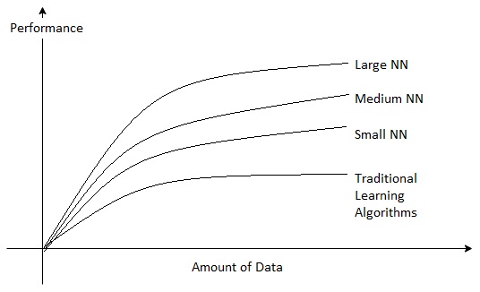
This picture clearly explains to us that, larger the neural network better the performance of the model is. One more thing to look closely at is, even after increasing the amount of data after a certain point, performance remains constant.

That was all the background you needed to get started with the actual working of an ANN.

Basics of Neural Network Programming :

The ANN is a complex and vast topic in itself, to begin with, first, we will try to understand what a Logistic regression is, we will try to get this by a simple Binary Classification (0, 1).

Let's say we are developing an algorithm to predict whether the given picture is a cat or not. The simple cat image which you see here is processed in the given format as the next picture on our computer.

Consider this picture as the first image in the training set

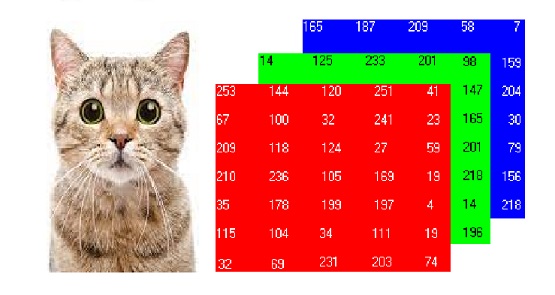
You might already know about it, each pixel in the picture of the cat has a particular value ranging from 0 to 255.

To process an image the computer stores them in these 3 channels – Red, Blue, and green. The image here looks (7 x 5 x 3)px, but actually, it isn’t. The real image might be (64 x 64 x 3)px, which means 64 rows and 64 columns of each red, blue and green and 3 channels of colors.

Before starting with Logistic Regression, first, let’s get familiar with the common notation used and needed for it.

Notation :

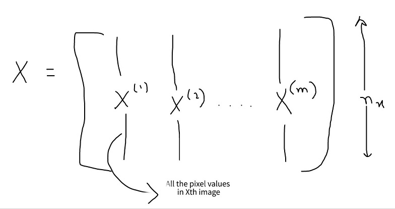
1. X -> this symbol is used to denote the matrix which consists of all the pixel values for a single image. (It is a column vector)

   X² = [253, 144, ... 14, 25, ... 165, 167 ... ] (this should be a column vector)

   = 64 x 64 x 3 = 12288

   = n = n_x = 12288 -> order = (12288 x 1) = (row x col)

2. The outputs are stored in Y which will be {0, 1} These outputs are the correct predictions for a picture, like if it is a cat then 1, if it isn’t then 0.

3. We will not be dealing with a single image but ‘m’ number of images. So.

$$
\begin{equation} Y = [y^1, y^2, y^3, … y^m] \end{equation} $$

$$
\begin{equation} (X, Y) \longrightarrow \hspace{1cm} X \in R^{n_{x}} , \hspace{1cm} Y \in [0, 1] \end{equation} $$

m training examples : $$
\begin{equation} [(x^{(1)}, y^{(1)}), (x^{(2)}, y^{(2)}) , (x^{(3)}, y^{(3)}) , … (x^{(m)}, y^{(m)})] \end{equation} $$

X.shape = $$
\begin{equation} (n_{x}, m) \end{equation} $$

Y.shape = $$
\begin{equation} (1, m) \end{equation} $$

Logistic Regression :

Logistic regression is a method adopted from statistics. This method deals with binary problems. it is a simple mathematical equation that takes an input and always results in the range (0, 1). So this is important for us in a way like if the value comes out to be greater than 0.5 then we consider that the prediction should be made 1, and if it results in 0.5 or less than 0.5 it should be predicted 0.

Yes, I know most of you would be like, what a picture of a cat has to do with something like logistic regression and how would we pass the image in a mathematical function. Don’t worry we will deal with all of these in few articles.

If you are worried about how to pass the image then remember we already know that images in computers are processed as a matrix of 3 dimensions. And also we have converted that 3-D matrix into a column vector. So It is possible.

The Logistic Regression In mathematical form is :

$$
\begin{equation} \sigma(z) = \frac{1}{1 + e^{-z}} \end{equation} $$

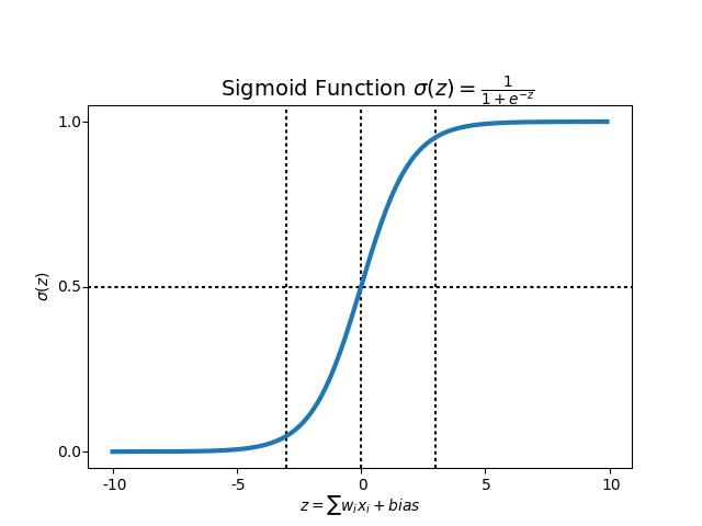
If z is large -> $$
\begin{equation} \sigma(z) = \frac{1}{1 + 0} = 1 \end{equation} $$

If z is large negative number -> $$
\begin{equation} \sigma(z) = \frac{1}{1 + \infty} = 0 \end{equation} $$

So now you have a brief idea about logistic regression and its application more importantly why we need it. Let’s get back to the Neural Network and try linking the logistic regression with it so that it makes more sense.

So this is how a neural network would look like a diagram.

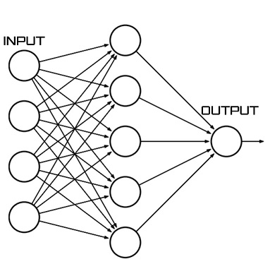
Each circle in the diagram is a neuron or a node. The first 4 nodes are called input features and the last one is the output. The layer of neurons in between is hidden layer.

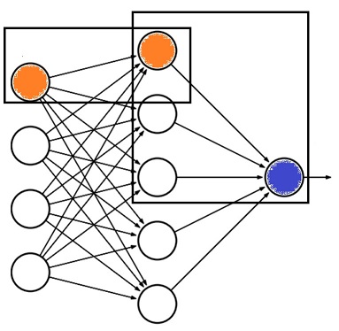
The orange neurons shown in the above diagram are the ones where the Logistic Regression cost function (is discussed in further articles) comes into action and the orange to blue neuron is the place where the sigmoid function comes into the action.

Working of a Neural Network with Logistic Regression :

As you already know about deep learning and up till now you have got an idea about logistic regression as well, let’s try to understand how neural networks work.

Each node to node neural network is a mathematical function that results in output and then these outputs are again passed into some another function to reach the final result. (This para might be confusing but you would get it more clear in further articles)

This idea of a neural network is all based on the solution to the simple mathematical equation of : $$
\begin{equation} \hat{y} = P(y=1|X) \end{equation} $$

which means, what is the probability of ŷ being 1, given X, where, ŷ is the probability of output being 1 and X is a matrix with all the images in pixels.

(Important paras ahead)

First, you need to make it very clear that this algorithm will not directly start predicting cats. You have to train this model on a certain number of images so that it can learn some patterns and then after training it would start predicting.

So now let's try to understand how the algorithm will learn the patterns and give an appropriate output. To begin with, first, the algorithm will take a training image to pass it through the neural network, predict it worse, and then it will make it go through a Logistic Regression cost function, which would determine how good our predicted output by the algorithm yhat is when the true label is y.

For the first time when we train a model we pass it both the image as well as the true label or the correct answer to the image so that the algorithm might correct itself every time it predicts a wrong output. This process of correction of the prediction is iterative within the model until the model predicts it correctly. With this repetitive prediction and correction, the model learns the patterns and gets better.

The term used for this iterative correction process is Back-propagation or backward propagation - helps to calculate the gradient of a loss function with respect to all the inputs in the network.

The Back-propagation function which we use in this case is :

Loss function :
$$
\begin{equation} L(\hat{y}, y) = -[y\log \hat{y} + (1-y)\log (1-y)] \end{equation} $$

Cost function :
$$
\begin{equation} J(w, b) = \frac{1}{m} \sum_{i=1}^{m} [ L(\hat{y}^i, y^i) ] \end{equation} $$

$$
\begin{equation} = - \frac{1}{m} \sum_{i=1}^{m} [ y^i\log \hat{y}^i + (1 - y^i)\log (1 - \hat{y}^i) ] \end{equation} $$

The loss function computes the error for a single training example; the cost function is the average of the loss functions of the entire training set.

One step of backward propagation on a computation graph yields derivative of final output variable.

This was all the theory needed for a, simple basic 1 layered Neural Network. In the next blog, we will discuss how to implement this in code using python.