Multi-Class CNN

For this next project in the series we will be dealing with a "multi-class" problem, where the classes to classify are more than 2 and in our case the data set we choose is the Fruits 262 available on Kaggle. Instead of this you can even choose a better arranged data, the Fruits 360 - A dataset with 90380 images of 131 fruits and vegetables.

The data in the initial stage is made ready with the help of Gerry's notebook on the similar problem.

This data set consists of 262 different types of fruits. This blog is more focused on the code, and covers only the explanation of the important code.

This blog is based on this project

The Kaggle API to import the data set in your notebook is :

kaggle datasets download -d aelchimminut/fruits262

If you don't know what above line means then please refer this

The repo for this blog also contains a helper_functions.py file, visit here - github.com/Hrushi11/Blogs-Repository/blob/m.., which will be made use throughout the notebook.

Importing Dependencies

Packages and modules required for successful running of this notebook.

# Importing dependencies
import os 
import random

import numpy as np
import pandas as pd
import matplotlib.pyplot as plt

import tensorflow as tf
from tensorflow.keras.layers.experimental import preprocessing
from tensorflow.keras.preprocessing.image import ImageDataGenerator

from sklearn.metrics import accuracy_score
from sklearn.metrics import classification_report
from sklearn.model_selection import train_test_split

from helper_functions import create_tensorboard_callback, plot_loss_curves, unzip_data, compare_historys, walk_through_dir, make_confusion_matrix

Getting our data ready

The data provided to us is a zip file so we will be unzipping the data set and have a look on the contents of our dataset. For this we will be using :

# Unzipping our data
unzip_data("/content/fruits262.zip")

# Check for dir in provided data
walk_through_dir("/content/Fruit-262")

Balancing the data

If we have a look on our data, we find that most of the image classes have uneven number of images which is not a good way for training the models since the model data should be bias free.

To overcome this problem we constraint all the image classes in the dataset to have only 200 images and dropping of all the image classes having less than 200 images per class.

After this, our dataset is reduced from 262 classes to 255 only.

# balancing the data allowing only similar number of images
dir="/content/Fruit-262"

filepaths=[]
labels=[]
classlist=os.listdir(dir)
for label in classlist:
    classpath=os.path.join(dir,label)
    if os.path.isdir(classpath):
        flist=os.listdir(classpath)
        for f in flist:
            fpath=os.path.join(classpath,f)
            filepaths.append(fpath)
            labels.append(label)                   
Fseries= pd.Series(filepaths, name='filepaths')
Lseries=pd.Series(labels, name='labels')    
df=pd.concat([Fseries, Lseries], axis=1)
print(df.head())
print(df['labels'].value_counts())

balance=df['labels'].value_counts()
blist=list(balance)
print(blist)

Converting the data into Data Frame

The data set given would be best to handle when converted into data frame. Also it becomes one of the way on passing the data to Image data generators.

# The data set given would be best to handle when converted into dataframe
print ('original number of classes: ', len(df['labels'].unique()))     
size=200 # set number of samples for each class
samples=[]
group=df.groupby(labels)
for label in df['labels'].unique():
    Lgroup=group.get_group(label)
    count=int(Lgroup['labels'].value_counts())    
    if count>=size:
        sample=Lgroup.sample(size, axis=0)
        samples.append(sample) 
df=pd.concat(samples, axis=0).reset_index(drop=True)
print (len(df))
print ('final number of classes: ', len(df['labels'].unique()))       
print (df['labels'].value_counts())

Splitting the dataset

The data set needs to split into train, test and validation so that we can evaluate our data bias free and in a better way.

# Getting dataframes ready for train, test and validation
train_split=.9
test_split=.05
dummy_split=test_split/(1-train_split)

train_df, dummy_df=train_test_split(df, 
                                    train_size=train_split, 
                                    shuffle=True, 
                                    random_state=123)

test_df, valid_df=train_test_split(dummy_df, 
                                   train_size=dummy_split, 
                                   shuffle=True, 
                                   random_state=123)

print ('train_df length: ', len(train_df), '  test_df length: ', len(test_df), '  valid_df length: ', len(valid_df))

Let's move ahead and create our Image Generators.

# Image generators
train_datagen = ImageDataGenerator()
val_datagen = ImageDataGenerator()
test_datagen = ImageDataGenerator()

Turning our data into batches

# Converting data ready into batches so that it is easier to train our model
train_data = train_datagen.flow_from_dataframe(train_df,
                                               x_col='filepaths',
                                               y_col='labels',
                                               target_size = (224, 224),
                                               batch_size = 32,
                                               seed=42,
                                               class_mode = 'categorical')

test_data = test_datagen.flow_from_dataframe(test_df,
                                             x_col='filepaths',
                                             y_col='labels',
                                             target_size = (224, 224),
                                             batch_size = 32,
                                             class_mode = 'categorical',
                                             shuffle=False)

val_data = test_datagen.flow_from_dataframe(valid_df,
                                            x_col='filepaths',
                                            y_col='labels',
                                            target_size = (224, 224),
                                            batch_size = 32,
                                            class_mode = 'categorical',
                                            shuffle=False)

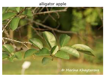
Viewing random image from our data set

# Viewing random image
files = pd.unique(train_df["filepaths"])
pic = random.choice(files)
img = plt.imread(pic)
pic = pic[19:]
plt.title(pic.split("/")[0])
plt.imshow(img)
plt.axis(False);

Data Augmentation Layer

Overfitting is one of the serious problems which we would encounter on working our ML projects. This is a condition in which the model learns the training data so well that it is not able to generalize well on the test data or the custom images given to it in the production.

There are many ways in which we can prevent overfitting, one of which we are using here is creating a data augmentation layer, a layer which would randomly resize, zoom or shift images in our training data, hence increasing the data set as well as increasing the chances of generalization for the model. The model comes up with different states of same images hence creating a variety for the same class with our manually adding more images to the dataset.

# Setting up augmentation layer
data_augmentation = tf.keras.models.Sequential([
  preprocessing.RandomFlip("horizontal"), 
  preprocessing.RandomRotation(0.2), 
  preprocessing.RandomHeight(0.2), 
  preprocessing.RandomWidth(0.2), 
  preprocessing.RandomZoom(0.2),
], name="data_augmentation_layer")

Model Building

A lot of different modelling techniques were tried before choosing this model structure and this a mere trial and error method for choosing a model and even fine tuning the number of layers.

You can always visit the ipython notebook for this blog (github.com/Hrushi11/Blogs-Repository/blob/m..) and find the code for the same here. But here we have the best model accuracy reached so far.

The best model is under Model 5 section in the ipython notebook.

# Setup base model and freeze its layers (this will extract features)
base_model = tf.keras.applications.EfficientNetB3(include_top=False)
base_model.trainable = False

# Setup model architecture with trainable top layers
inputs = tf.keras.layers.Input(shape=(224, 224, 3), name="input_layer") 
x = data_augmentation(inputs) 
x = base_model(x, training=False) 
x = tf.keras.layers.GlobalAveragePooling2D(name="global_average_pooling")(x) 
outputs = tf.keras.layers.Dense(255, activation="softmax", name="output_layer")(x) 
model_B3 = tf.keras.Model(inputs, outputs)

# Compile
model_B3.compile(loss="categorical_crossentropy",
                 optimizer=tf.keras.optimizers.Adam(),
                 metrics=["accuracy"])

# Fit
history_B3 = model_B3.fit(train_data,
                          epochs=5,
                          steps_per_epoch=len(train_data), 
                          validation_data=val_data,
                          validation_steps=len(val_data))

For this case we are using EfficientNetB3 one of the models in line with the EfficientNet series. One of the important points to remember before using the EfficientNet model is that it has a pre-trained Normalization layer and hence need not to be written explicitly. On the other hand if you use any other type of model there is a high chance that you would have to Normalize the input features for the betterment of the model.

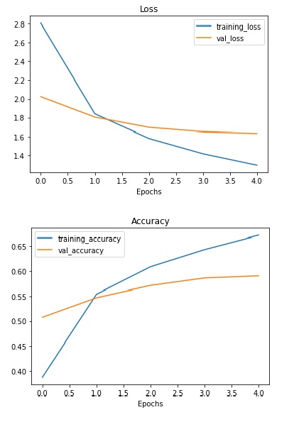
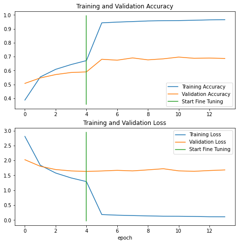
The maximum accuracy reached here is 59.02% on the validation data. Let's fine tune the model and further try to leverage this accuracy.

For this case we will be unfreezing the last 50 layers of the model and using a lower adam learning rate so that it doesn't skips the minima.

# Unfreeze all of the layers in the base model
base_model.trainable = True

# Refreeze every layer except for the last 50
for layer in base_model.layers[:-50]:
  layer.trainable = False

# Recompile model with lower learning rate
model_B3.compile(loss='categorical_crossentropy',
                 optimizer=tf.keras.optimizers.Adam(1e-4),
                 metrics=['accuracy'])

early_stopping = tf.keras.callbacks.EarlyStopping(monitor="val_accuracy",
                                                  patience=3)

# Fine-tune for 45 more epochs (5+45)
fine_tune_epochs = 50

history_B3_fine_tune_1 = model_B3.fit(train_data,
                                      epochs=fine_tune_epochs,
                                      validation_data=val_data,
                                      validation_steps=len(val_data),
                                      initial_epoch=history_B3.epoch[-1],
                                      callbacks=early_stopping)

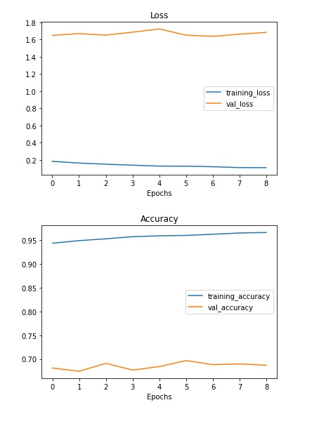
The validation accuracy now reached is 68.71% which is far more than guessing on 255 classes of images.

Viewing the loss curves

1. For the first 5 epochs :

2. For the next 8 epochs :

3. For the remaining epochs :

Saving the model

Saving this model in the drive so that we need not to retrain the parameters and get the weights

tf.keras.models.save_model(model_B3, "/content/drive/MyDrive/Fruits-262_Model")

model_load = tf.keras.models.load_model("/content/drive/MyDrive/Fruits-262_Model")

Evaluation of the best model

Insights of the best Model

Let's have some insights on how the model has predicted on the test data like the number of prediction probability for each class and having a look on confusion matrix and F1 score graph.

Most of the important insights lies in the code and so I would recommend you to read it from (github.com/Hrushi11/Blogs-Repository/blob/m..) under the section Insights of the best Model.

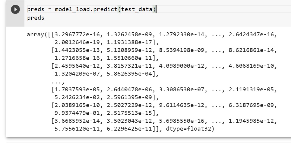
Looking at the prediction probabilities:

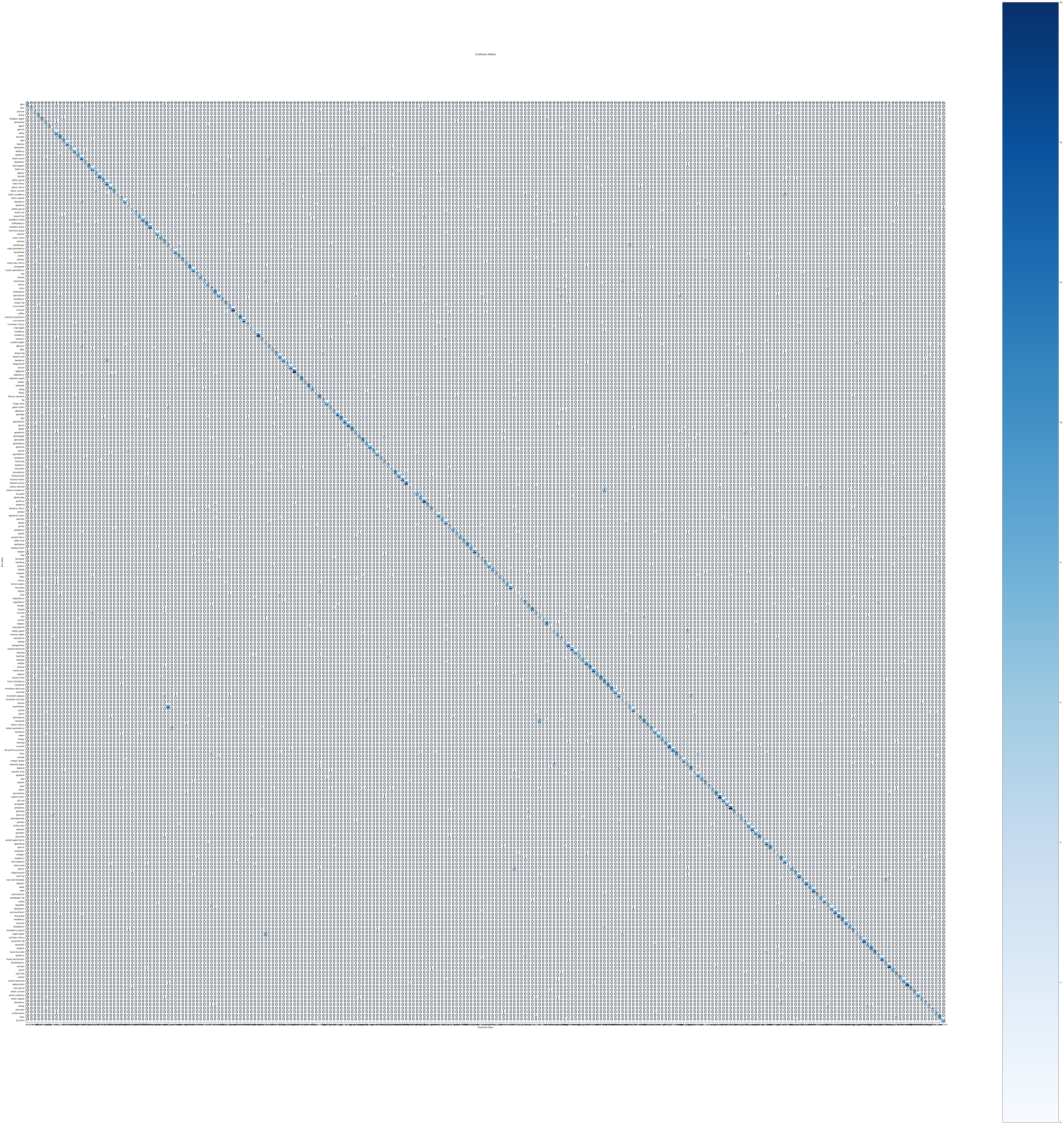
Confusion Matrix

The Confusion matrix shown here is hard to read and study but if you try to zoom and try to see the numbers then we actually get to know what are the classes which are getting confused with each other.

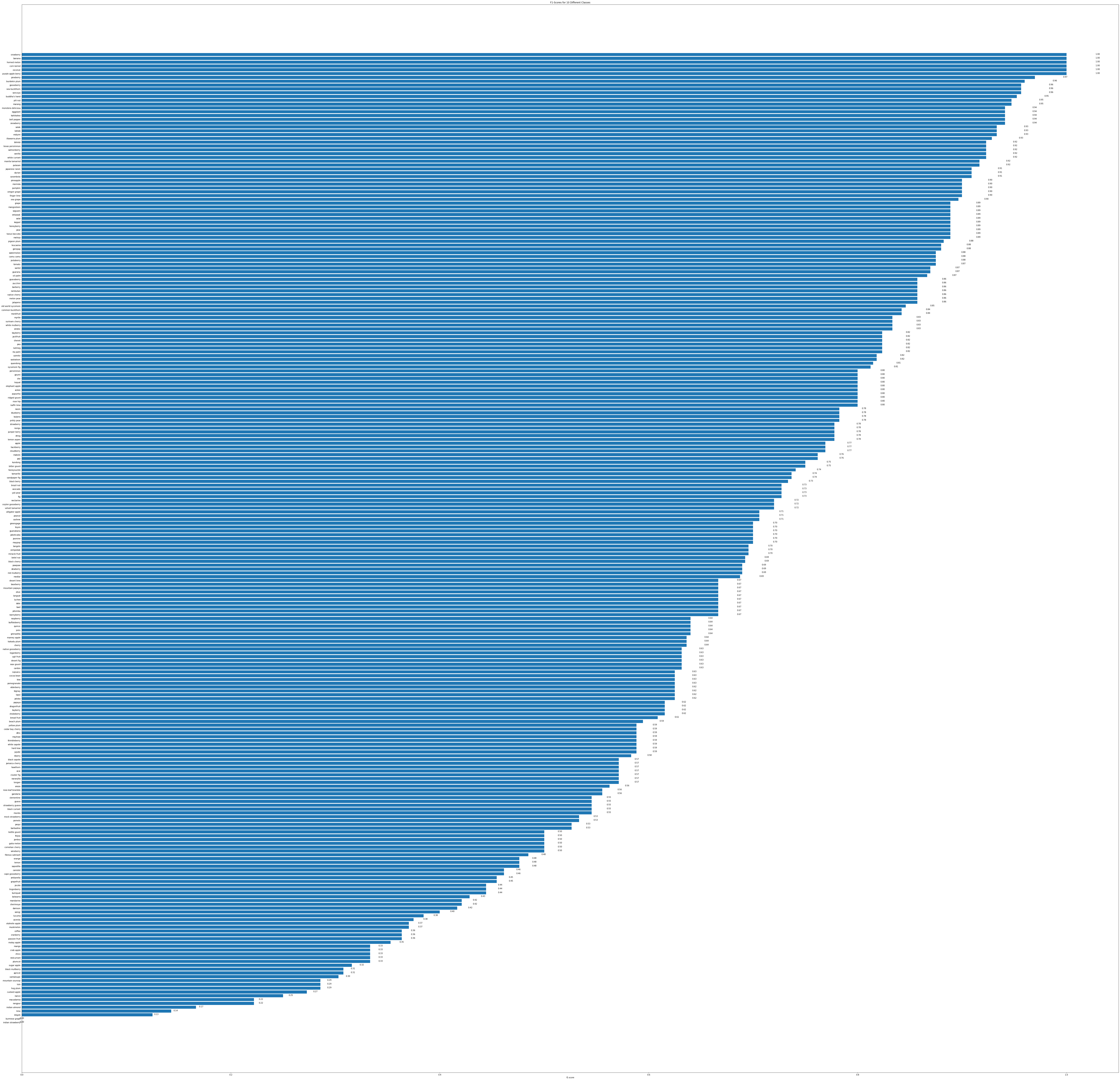
F1 score graph

F1 is another metrics which is most commonly used to evaluate the data we get insights through this as well.

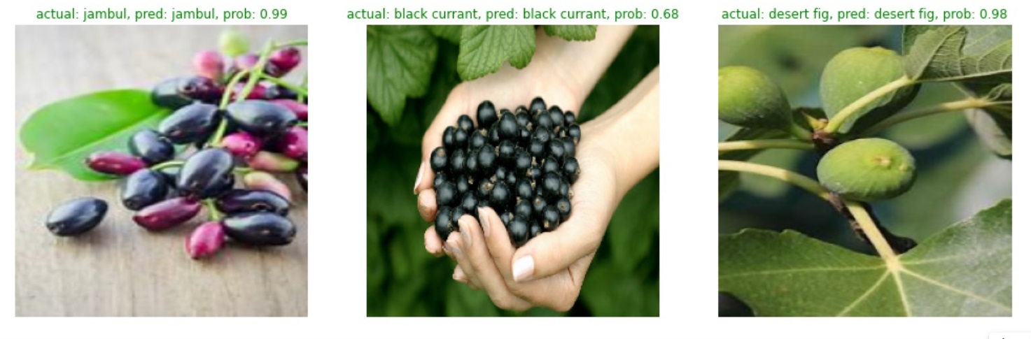
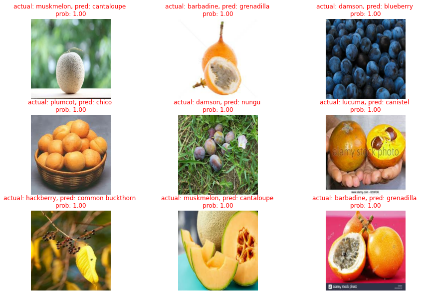
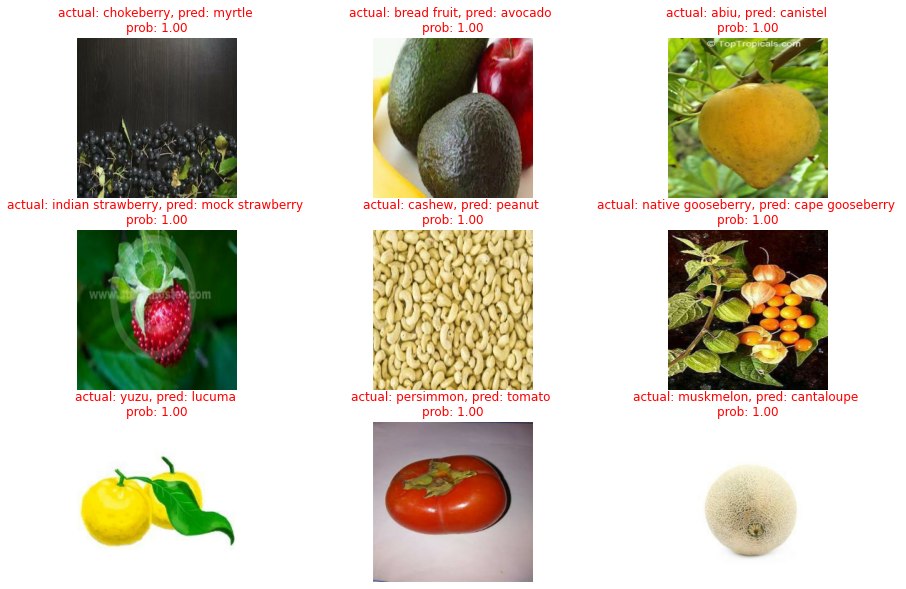
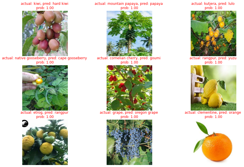
Visualizing the wrong predictions

This section is very important since we might get to know the actual reasons for why the image might be predicted wrong some of the visuals are shown here.

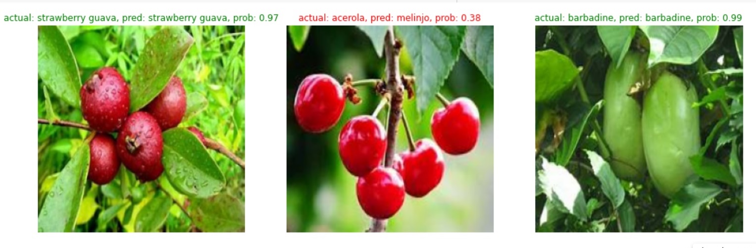
Look on wrong images

The images which were altogether predicted wrong on the test data were. The codes are all available (github.com/Hrushi11/Blogs-Repository/blob/m..)

Conclusion

This was all for this project, congratulations on coming this far, training neural nets is never a difficult task but to scale up the same neural network so that it performs well on the dataset is quite a tedious process and is enhanced with time.

So even though the project is closed from my side, you can increase the accuracy by different methods and let me know with the connection links available at the top.

Happy scaling up!