Programming Neural Networks :

In the last blog, we discussed the theoretical aspects of Neural Networks. We discussed important points like what are Neural Networks and why they are important, also how they work.

In this blog, we will be dealing with the practical aspects of Neural Networks and try to program and run a simple neural network. To begin with, you should already have some pre-requisites as mentioned here.

Must be familiar with Jupyter Notebooks.

Must be familiar with python libraries Numpy and Matplotlib.

If you are good with these then we are good to go.

Most of the time you will find that ML engineers use ‘Numpy’ since NumPy arrays are faster and more compact than Python lists.

In this blog, we will build a simple image-recognition algorithm that can correctly classify pictures as cat or non-cat.

All the files related to this blog as well as the ipython notebook is available on my Github

Logistic Regression :

To begin our programming first we will code a simple Logistic regression algorithm and then move forward to code a single-layered Neural network.

Coding a model consists of :

Initialize the parameters of the model
Learn the parameters for the model by minimizing the cost
Use the learned parameters to make predictions (on the test set)
Analyse the results and conclude

The steps required to proceed are:

Define the model structure (such as the number of input features)
Initialize the model's parameters
Loop :

Calculate current loss (forward propagation)
Calculate current gradient (backward propagation)
Update parameters (gradient descent)

We will be creating separate functions for each of these and then combine all of the functions and name that combined function model(). Which will be our Logistic regression.

The libraries we will need to import will be:

import numpy as np
import matplotlib.pyplot as plt
import h5py
import scipy
from PIL import Image
from scipy import ndimage
import os

%matplotlib inline

Getting the dataset ready

To be able to code our model we will need a dataset, download these files from here and change the <your_train_file_path> with the location of train_catvnoncat.h5 file on your local device.

To load the dataset :

def load_dataset():
    train_dataset = h5py.File('<your_train_file_path>', "r") # Change the file path
    train_set_x_orig = np.array(train_dataset["train_set_x"][:]) # your train set features
    train_set_y_orig = np.array(train_dataset["train_set_y"][:]) # your train set labels

    test_dataset = h5py.File('<your_test_file_path>', "r") # Change the file path
    test_set_x_orig = np.array(test_dataset["test_set_x"][:]) # your test set features
    test_set_y_orig = np.array(test_dataset["test_set_y"][:]) # your test set labels

    classes = np.array(test_dataset["list_classes"][:]) # the list of classes

    train_set_y_orig = train_set_y_orig.reshape((1, train_set_y_orig.shape[0]))
    test_set_y_orig = test_set_y_orig.reshape((1, test_set_y_orig.shape[0]))

    return train_set_x_orig, train_set_y_orig, test_set_x_orig, test_set_y_orig, classes

load_dataset()

Now, splitting the dataset into training and test set :

train_set_x_orig, train_set_y, test_set_x_orig, test_set_y, classes = load_dataset()

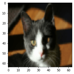
Visualizing a random image from our dataset :

# Example of a picture
index = 19
plt.imshow(train_set_x_orig[index])
print ("y = " + str(train_set_y[:,index]) + ", it's a '" + classes[np.squeeze(train_set_y[:,index])].decode("utf-8") +  "' picture.")

This outputs :

For convenience, we should now reshape images of shape (num_px, num_px, 3) in a numpy-array of shape (num_px * num_px * 3, 1). After this, our training (and test) dataset is a numpy-array where each column represents a flattened image. There should be m_train (respectively m_test) columns.

# Reshape the training and test examples

train_set_x_flatten = train_set_x_orig.reshape(train_set_x_orig.shape[0], -1).T
test_set_x_flatten = test_set_x_orig.reshape(test_set_x_orig.shape[0], -1).T

print ("train_set_x_flatten shape: " + str(train_set_x_flatten.shape))
print ("train_set_y shape: " + str(train_set_y.shape))
print ("test_set_x_flatten shape: " + str(test_set_x_flatten.shape))
print ("test_set_y shape: " + str(test_set_y.shape))
print ("sanity check after reshaping: " + str(train_set_x_flatten[0:5,0]))

One common preprocessing step in machine learning is to center and standardize your dataset, meaning that you substract the mean of the whole numpy array from each example, and then divide each example by the standard deviation of the whole numpy array. But for picture datasets, it is simpler and more convenient and works almost as well to just divide every row of the dataset by 255 (the maximum value of a pixel channel).

Let's standardize our dataset.

train_set_x = train_set_x_flatten / 255.
test_set_x = test_set_x_flatten / 255.

We are trying to build a logistic regression model so the first helper function we will need is a sigmoid function :

The Logistic Regression In mathematical form is :

$$
\begin{equation} \sigma(z) = \frac{1}{1 + e^{-z}} \end{equation} $$

# SIGMOID FUNCTION

def sigmoid(z):
    s = 1 / (1 + np.exp(-z))
    return s

Initializing Parameters : We have to initialize w as a vector of zeros.

# initialize_with_zeros
def initialize_with_zeros(dim):

    w = np.zeros(shape=(dim, 1))
    b = 0

    assert(w.shape == (dim, 1))
    assert(isinstance(b, float) or isinstance(b, int))

    return w, b

Forward and Backward propagation :

Now that our parameters are initialized, we can do the "forward" and "backward" propagation steps for learning the parameters.

Let's implement a function propagate() that computes the cost function and its gradient.

# propagate

def propagate(w, b, X, Y):

    m = X.shape[1]

    # FORWARD PROPAGATION (FROM X TO COST)
    A = sigmoid(np.dot(w.T, X) + b)  # compute activation
    cost = (- 1 / m) * np.sum(Y * np.log(A) + (1 - Y) * (np.log(1 - A)))  # compute cost

    # BACKWARD PROPAGATION (TO FIND GRAD)
    dw = (1 / m) * np.dot(X, (A - Y).T)
    db = (1 / m) * np.sum(A - Y)

    assert(dw.shape == w.shape)
    assert(db.dtype == float)
    cost = np.squeeze(cost)
    assert(cost.shape == ())

    grads = {"dw": dw,
             "db": db}

    return grads, cost

Optimization : To update the parameters using gradient descendant.

# GRADED FUNCTION: optimize

def optimize(w, b, X, Y, num_iterations, learning_rate, print_cost = False):

    costs = []

    for i in range(num_iterations):


        # Cost and gradient calculation (≈ 1-4 lines of code)
        grads, cost = propagate(w, b, X, Y)

        # Retrieve derivatives from grads
        dw = grads["dw"]
        db = grads["db"]

        # update rule (≈ 2 lines of code)
        w = w - learning_rate * dw  # need to broadcast
        b = b - learning_rate * db

        # Record the costs
        if i % 100 == 0:
            costs.append(cost)

        # Print the cost every 100 training examples
        if print_cost and i % 100 == 0:
            print ("Cost after iteration %i: %f" % (i, cost))

    params = {"w": w,
              "b": b}

    grads = {"dw": dw,
             "db": db}

    return params, grads, costs

Prediction : To predict

Calculate $$ \hat{Y} = A = \sigma(w^T X + b) $$

Converting the entries of a into 0 (if activation <= 0.5) or 1 (if activation > 0.5), stores the predictions in a vector Y_prediction.

# GRADED FUNCTION: predict

def predict(w, b, X):

    m = X.shape[1]
    Y_prediction = np.zeros((1, m))
    w = w.reshape(X.shape[0], 1)

    # Compute vector "A" predicting the probabilities of a cat being present in the picture
    ### START CODE HERE ### (≈ 1 line of code)
    A = sigmoid(np.dot(w.T, X) + b)

    for i in range(A.shape[1]):
        # Convert probabilities a[0,i] to actual predictions p[0,i]
        ### START CODE HERE ### (≈ 4 lines of code)
        Y_prediction[0, i] = 1 if A[0, i] > 0.5 else 0

    assert(Y_prediction.shape == (1, m))

    return Y_prediction

Merging all functions into a model : `model()`

# GRADED FUNCTION: model

def model(X_train, Y_train, X_test, Y_test, num_iterations=2000, learning_rate=0.5, print_cost=False):

    # initialize parameters with zeros (≈ 1 line of code)
    w, b = initialize_with_zeros(X_train.shape[0])

    # Gradient descent (≈ 1 line of code)
    parameters, grads, costs = optimize(w, b, X_train, Y_train, num_iterations, learning_rate, print_cost)

    # Retrieve parameters w and b from dictionary "parameters"
    w = parameters["w"]
    b = parameters["b"]

    # Predict test/train set examples (≈ 2 lines of code)
    Y_prediction_test = predict(w, b, X_test)
    Y_prediction_train = predict(w, b, X_train)

    # Print train/test Errors
    print("train accuracy: {} %".format(100 - np.mean(np.abs(Y_prediction_train - Y_train)) * 100))
    print("test accuracy: {} %".format(100 - np.mean(np.abs(Y_prediction_test - Y_test)) * 100))


    d = {"costs": costs,
         "Y_prediction_test": Y_prediction_test, 
         "Y_prediction_train" : Y_prediction_train, 
         "w" : w, 
         "b" : b,
         "learning_rate" : learning_rate,
         "num_iterations": num_iterations}

    return d

To Train our model :

d = model(train_set_x, train_set_y, test_set_x, test_set_y, num_iterations = 2000, learning_rate = 0.005, print_cost = True)

It should look something like this after running

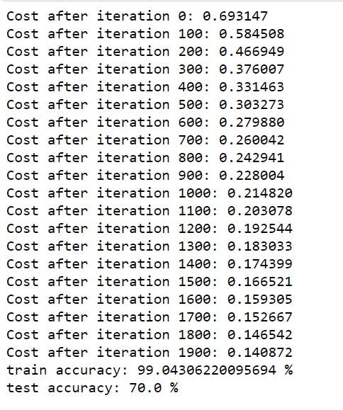
The training accuracy is 100% which means our model is overfitting the training data, but no worries we will learn regularization in future which will take care of this.

The test accuracy is 70% which is not quite good but still this being just a logistic regression model it is worth, In the future blogs, when we will train actual Neural networks these scores will be more digestable.

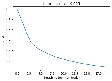
The Learning rate is :

# Plot learning curve (with costs)
costs = np.squeeze(d['costs'])
plt.plot(costs)
plt.ylabel('cost')
plt.xlabel('iterations (per hundreds)')
plt.title("Learning rate =" + str(d["learning_rate"]))
plt.show()

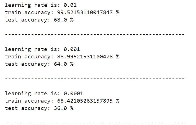
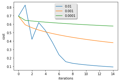
Choice of learning rate :

In order for Gradient Descent to work we must choose the learning rate wisely. The learning rate α determines how rapidly we update the parameters. If the learning rate is too large we may "overshoot" the optimal value. Similarly, if it is too small we will need too many iterations to converge to the best values. That's why it is crucial to use a well-tuned learning rate.

Let's compare the learning curve of our model with several choices of learning rates. Run the cell below. This should take about 1 minute

learning_rates = [0.01, 0.001, 0.0001]
models = {}
for i in learning_rates:
    print ("learning rate is: " + str(i))
    models[str(i)] = model(train_set_x, train_set_y, test_set_x, test_set_y, num_iterations = 1500, learning_rate = i, print_cost = False)
    print ('\n' + "-------------------------------------------------------" + '\n')

for i in learning_rates:
    plt.plot(np.squeeze(models[str(i)]["costs"]), label= str(models[str(i)]["learning_rate"]))

plt.ylabel('cost')
plt.xlabel('iterations')

legend = plt.legend(loc='upper center', shadow=True)
frame = legend.get_frame()
frame.set_facecolor('0.90')
plt.show()

So, now we are done with all the training and analysis of our model, let's code some more to get our model ready for predicting on custom images.

Before moving with the next lines of code please make sure your environment has imageio and scipy==1.1.0 libraries install if not:

pip install imageio

pip install scipy==1.1.0

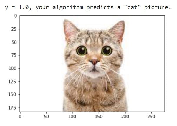
Predictions on custom images :

To predict on custom images change the fname variable with your image path on your local device.

import imageio

# preprocessing the image to fit our algorithm.
fname = "<your_custom_path>" # Change this
image = np.array(imageio.imread(fname))
my_image = scipy.misc.imresize(image, size=(num_px, num_px)).reshape((1, num_px * num_px * 3)).T
my_predicted_image = predict(d["w"], d["b"], my_image)

plt.imshow(image)
print("y = " + str(np.squeeze(my_predicted_image)) + ", your algorithm predicts a \"" + classes[int(np.squeeze(my_predicted_image)),].decode("utf-8") +  "\" picture.")

I trained it on my custom image and got this result, try with non-cat images and see what the model predicts.

So, finally we are done with programming our logistic regression model to predict whether an image is a cat or not.

All of the code discussed here in the blog is available - here

In our next blog we will train an actual Neural Network model with hidden layers.

So stay connected.

Programming Neural Networks

A beginner friendly blog for people who want to train there first Neural Network.