TensorFlow, a deeplearning framework

Tensorflow is a deeplearning framework used to train deeplearning models easily which is opensource and maintained by google.

This notebook deals with training an end to end neural network. We can train a neural network just by using the numpy library but that's a long and tedious process so for to make this easier we will use tensorflow with the latest version.

For this notebook we will build a simple hand sign classifier with the help of a 3 layered neural network.

Data is available - here

ipython notebook for this blog - here

# Check for tensorflow version
import tensorflow as tf
tf.__version__

# importing libraries we will need
import h5py
import numpy as np
import time
import matplotlib.pyplot as plt

Getting our data ready

For this blog our dataset is present in a h5py file, let's get it ready so that we can use it.

train_dataset = h5py.File('/content/drive/MyDrive/dataset/train_signs.h5', "r")
test_dataset = h5py.File('/content/drive/MyDrive/dataset/test_signs.h5', "r")

Here we will call the TensorFlow dataset created on a HDF5 file, which we can use in place of a Numpy array to store our datasets.

x_train = tf.data.Dataset.from_tensor_slices(train_dataset['train_set_x'])
y_train = tf.data.Dataset.from_tensor_slices(train_dataset['train_set_y'])

x_test = tf.data.Dataset.from_tensor_slices(test_dataset['test_set_x'])
y_test = tf.data.Dataset.from_tensor_slices(test_dataset['test_set_y'])

# Check for the type
type(x_train)

TensorFlow Datasets are generators, we can't access directly the contents unless we iterate over them in a for loop. Let's do this by using a iter and next in python.

print(next(iter(x_train)))

# check for details in y_train
print(y_train.element_spec)

Normalizing function

Now, let's create a function which normalizes our images like converts them into tensors and in the dimension (64 x 64 x 3, 1).

To apply this function to each element we will use map() function.

def normalize(image):

    image = tf.cast(image, tf.float32) / 256.0
    image = tf.reshape(image, [-1,1])
    return image

# applying the function to each image 
new_train = x_train.map(normalize)
new_test = x_test.map(normalize)

new_train.element_spec

x_train.element_spec

print(next(iter(new_train)))

One Hot Encodings

In deeplearning sometimes we come accross some of the problems where the y mappings are not just classified between two(0, 1) but different. And hence to convert this into (0, 1) we use one_hot_encoding.

This is called "one hot" encoding, because in the converted representation, exactly one element of each column is "hot" (meaning set to 1)

def one_hot_matrix(label, depth=6):
    one_hot = tf.reshape(tf.one_hot(label, depth, axis=0), (depth,1))

    return one_hot

new_y_test = y_test.map(one_hot_matrix)
new_y_train = y_train.map(one_hot_matrix)

print(next(iter(new_y_test)))

Initializing the parameters

Now we'll initialize a vector of numbers between zero and one.

The function we are using is - tf.keras.initializers.GlorotNormal(seed=1) - we are using a seed here so that the initializer always comes up with the same random values.

This function draws samples from a truncated normal distribution centered on 0, with stddev = sqrt(2 / (fan_in + fan_out)), where fan_in is the number of input units and fan_out is the number of output units, both in the weight tensor.

Initializing parameters to build a neural network with TensorFlow. The shapes are:
W1 : [25, 12288]
b1 : [25, 1]
W2 : [12, 25]
b2 : [12, 1]
W3 : [6, 12]
b3 : [6, 1]

def initialize_parameters():

    initializer = tf.keras.initializers.GlorotNormal(seed=1)   

    W1 = tf.Variable(initializer(shape=(25, 12288)))
    b1 = tf.Variable(initializer(shape=(25, 1)))
    W2 = tf.Variable(initializer(shape=(12, 25)))
    b2 = tf.Variable(initializer(shape=(12, 1)))
    W3 = tf.Variable(initializer(shape=(6, 12)))
    b3 = tf.Variable(initializer(shape=(6, 1)))

    parameters = {"W1": W1,
                  "b1": b1,
                  "W2": W2,
                  "b2": b2,
                  "W3": W3,
                  "b3": b3}

    return parameters

Two most important steps :

1. Implement forward propagation
   
2. Retrieve the gradients and train the model

We are training our model with tensorflow and while using it we have this benefit of not using the backpropagation as tensorflow takes care of it for us. This is also the reason why tensorflow is a great deeplearning framework.

We need to only work on forward propagation.

Here, we'll use a TensorFlow decorator, @tf.function, which builds a computational graph to execute the function. @tf.function is polymorphic, which comes in very handy, as it can support arguments with different data types or shapes, and be used with other languages, such as Python. This means that you can use data dependent control flow statements.

When you use @tf.function to implement forward propagation, the computational graph is activated, which keeps track of the operations. This is so you can calculate your gradients with backpropagation.

Implementing the forward propagation for the model: LINEAR -> RELU -> LINEAR -> RELU -> LINEAR

@tf.function
def forward_propagation(X, parameters):

    # Retrieve the parameters from the dictionary "parameters" 
    W1 = parameters['W1']
    b1 = parameters['b1']
    W2 = parameters['W2']
    b2 = parameters['b2']
    W3 = parameters['W3']
    b3 = parameters['b3']

    Z1 = tf.math.add(tf.linalg.matmul(W1, X), b1)
    A1 = tf.keras.activations.relu(Z1)
    Z2 = tf.math.add(tf.linalg.matmul(W2, A1), b2)
    A2 = tf.keras.activations.relu(Z2)
    Z3 = tf.math.add(tf.linalg.matmul(W3, A2), b3)

    return Z3

Computing the cost

Here again, @tf.function decorator steps in and saves us time. All we need to do is specify how to compute the cost, and we can do so in one simple step by using:

tf.reduce_mean(tf.keras.losses.binary_crossentropy(y_true = ..., y_pred = ..., from_logits=True))

@tf.function
def compute_cost(logits, labels):

    cost = tf.reduce_mean(tf.keras.losses.binary_crossentropy(y_true = labels, y_pred = logits, from_logits=True))

    return cost

Training the model

Almost all of our functions are ready to use in the model except the deciding the optimizer which we will decide in the model() function. For this case we are using SGD - stochastic gradient descent.

The tape.gradient function: this allows us to retrieve the operations recorded for automatic differentiation inside the GradientTape block. Then, calling the optimizer method apply_gradients, will apply the optimizer's update rules to each trainable parameter.

tf.Data.dataset = dataset.prefetch(8) - What this does is prevent a memory bottleneck that can occur when reading from disk. prefetch() sets aside some data and keeps it ready for when it's needed. It does this by creating a source dataset from your input data, applying a transformation to preprocess the data, then iterating over the dataset the specified number of elements at a time. This works because the iteration is streaming, so the data doesn't need to fit into the memory.

def model(X_train, Y_train, X_test, Y_test, learning_rate = 0.0001,
          num_epochs = 1500, minibatch_size = 32, print_cost = True):

    costs = []                                        # To keep track of the cost

    # Initializing our parameters
    parameters = initialize_parameters()

    W1 = parameters['W1']
    b1 = parameters['b1']
    W2 = parameters['W2']
    b2 = parameters['b2']
    W3 = parameters['W3']
    b3 = parameters['b3']

    # Optimizer selection
    optimizer = tf.keras.optimizers.SGD(learning_rate)

    X_train = X_train.batch(minibatch_size, drop_remainder=True).prefetch(8)# <<< extra step    
    Y_train = Y_train.batch(minibatch_size, drop_remainder=True).prefetch(8) # loads memory faster 

    # Do the training loop
    for epoch in range(num_epochs):

        epoch_cost = 0.

        for (minibatch_X, minibatch_Y) in zip(X_train, Y_train):
            # Select a minibatch
            with tf.GradientTape() as tape:
                # 1. predict
                Z3 = forward_propagation(minibatch_X, parameters)
                # 2. loss
                minibatch_cost = compute_cost(Z3, minibatch_Y)

            trainable_variables = [W1, b1, W2, b2, W3, b3]
            grads = tape.gradient(minibatch_cost, trainable_variables)
            optimizer.apply_gradients(zip(grads, trainable_variables))
            epoch_cost += minibatch_cost / minibatch_size

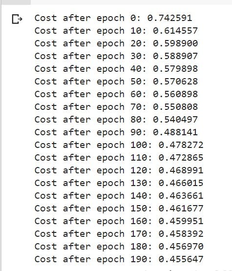
        # Print the cost every epoch
        if print_cost == True and epoch % 10 == 0:
            print ("Cost after epoch %i: %f" % (epoch, epoch_cost))
        if print_cost == True and epoch % 5 == 0:
            costs.append(epoch_cost)

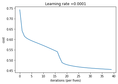
    # Plot the cost
    plt.plot(np.squeeze(costs))
    plt.ylabel('cost')
    plt.xlabel('iterations (per fives)')
    plt.title("Learning rate =" + str(learning_rate))
    plt.show()

    # Save the parameters in a variable
    print ("Parameters have been trained!")

    return parameters

# training the model on the data set 
model(new_train, new_y_train, new_test, new_y_test, num_epochs=200)

So, we are done with our building a 3 layered neural network with tensorflow.